This post finishes the discussion on Neural Samplers for Variational Inference by introducing some recent results (including mine).

Also, there's a talk recording of me presenting this post's content, so if you like videos more than texts, check it out.

Quick Recap

It all started with an aspiration for a more expressive variational approximation $q_\phi(z|x)$ since it restricts expressivity of our hierarhical model $p_\theta(x)$. We could use the multisample bound, which can lighten the restriction to an arbitrary extent, but the price is more computation and multiple evaluations of high-dimensional decoder $p_\theta(x|z)$ are especially frustrating.

Instead, we hope to leverage Neural Net's universal approximation properties and introduce a hierarchical variational approximation $q_\phi(z|x) = \int q_\phi(z, \psi|x) d\psi$ which should be much more expressive and we can sample from it by passing some simple noise $\psi$ through a neural network that generates¹ $q_\phi(z|\psi, x)$ distribution. However, we lost access to the marginal log-density $\log q_\phi(z|x)$, required by the KL term of the ELBO.

A theoretically sound way then is to give an upper bound on the log-density (to obtain a lower bound on the ELBO), but this bound regularizes the $q_\phi(z|x)$ and alleviating this regularization requires more expressive auxiliary variational distribution $\tau_\eta(\psi|x,z)$. Full circle, full stop. At this point, an efficiently computable multisample variational upper bound on the $\log q_\phi(z|x)$ would be handy, but our naive attempt to obtain one was unsuccessful. Moreover, it might well be that there are no good bounds at all.

~~New~~ Semi-Implicit Hope

A year ago Mingzhang Yin and Mingyuan Zhou published a paper Semi-Implicit Variational Inference (SIVI) where they essentially proposed the following multisample surrogate ELBO for our model:

$$ \hat{\mathcal{L}}_K^\text{SIVI} := \E_{q_\phi(z, \psi_0|x)} \E_{q_\phi(\psi_{1:K}|x)} \log \frac{p_\theta(x, z)}{ \frac{1}{K+1} \sum_{k=0}^K q_\phi(z|\psi_k, x) } $$

However, the original paper did not prove that this surrogate is a lower bound for all finite $K$, only that it converges to the ELBO $\mathcal{L}$ in the limit of infinite $K$. This fact was later shown by Molchanov et al.: this surrogate objective is indeed a lower bound for all finite $K$. Moreover, since this is a lower bound on ELBO,

$$ \E_{q_\phi(z, \psi_0|x)} \E_{q_\phi(\psi_{1:K}|x)} \left[ \log \frac{p_\theta(x, z)}{ q_\phi(z|x) } - \log \frac{p_\theta(x, z)}{ \frac{1}{K+1} \sum_{k=0}^K q_\phi(z|\psi_k, x) } \right] \ge 0 $$ We can recover an upper bound on the marginal log-density (at least in expectation) $$ \E_{q_\phi(z|x)} \log q_\phi(z|x) \le \E_{q_\phi(z|x)} \E_{q_\phi(\psi_0|z, x)} \E_{q_\phi(\psi_{1:K}|x)} \log \frac{1}{K+1} \sum_{k=0}^K q_\phi(z|\psi_k, x) $$

Which does indeed give us a multisample upper bound (not variational, though). Unfortunately, this particular bound has a severe weakness: the samples $\psi_{1:K}$ are uninformed about the $z$ they're supposed to describe in the $q(z|x,\psi_k)$ terms, so they are likely to do a poor job of reconstructing a particular $z$.

Interestingly, this bound looks similar to the multisample variational lower bound $\mathcal{L}_K$... $$ \log q(z|x) \ge \E_{\tau_\eta(\psi_{1:K}|z, x)} \log \frac{1}{K} \sum_{k=1}^K \frac{q_\phi(z, \psi_k|x)}{\tau_\eta(\psi_k|x,z)} $$ ... when $\tau_\eta(\psi|x,z)$ is taken to be $q_\phi(\psi|x)$ -- the "variational prior": $$ \log q(z|x) \ge \E_{q_\phi(\psi_{1:K}|x)} \log \frac{1}{K} \sum_{k=1}^K q_\phi(z|\psi_k, x) $$

The only difference between this lower bound and the SIVI upper bound is that the later adds one (free, see previous post for the discussion on free posterior samples) sample from the true inverse model $q_\phi(\psi|x,z)$.

Importance Weighted Hierarchical Variational Inference

The natural question to ask then is... could maybe the following be an upper bound on $\log q_\phi(z|x)$? $$ \mathcal{U}_K := \E_{q_\phi(\psi_0|z, x)} \E_{\tau_\eta(\psi_{1:K}|z, x)} \log \frac{1}{K+1} \sum_{k=0}^K \frac{q_\phi(z, \psi_k|x)}{\tau_\eta(\psi_k|x,z)} $$ The formula is very bizarre, yet several special cases do give upper bounds:

• Setting $K=0$ gives the Hierarchical Variational Models (HVM) bound (from the previous post) for arbitrary $\tau_\eta(\psi|x,z)$,
• Setting $\tau_\eta(\psi|x,z) = q_\phi(\psi|x)$ gives the SIVI bound for arbitrary $K$,
• Setting $\tau_\eta(\psi|x,z) = q_\phi(\psi|{\color{red} z}, x)$ recovers the $\log q_\phi(z|x)$ exactly.

The Importance Weighted Hierarchical Variational Inference paper gives an affirmative answer. $\mathcal{U}_K$ is indeed an upper bound (Multisample Variational Upper Bound) for any $K$ and any $\tau(\psi|x,z)$. Moreover, it enjoys same guarantees as the IWAE bound (Multisample Variational Lower Bound):

1. $\mathcal{U}_K \ge \log q_\phi(z|x)$
2. $\mathcal{U}_K \ge \mathcal{U}_{K+1}$
3. $\lim_{K \to \infty} \mathcal{U}_K = \log q_\phi(z|x)$

Combining this bound with the (intractable) ELBO, we obtain the following lower bound on $\log p_\theta(x)$:

$$ \hat{\mathcal{L}}_K^\text{IWHVI} := \E_{q_\phi(z, \psi_0|x)} \E_{\tau_\eta(\psi_{1:K}|z, x)} \log \frac{p_\theta(x, z)}{ \frac{1}{K+1} \sum_{k=0}^K \frac{q_\phi(z, \psi_k|x)}{\tau_\eta(\psi_k|x,z)} } $$

To test the bound we used a simple toy task of upper-bounding the negative differential entropy $\mathbb{E}_{q(z)} \log q(z)$ of the standard 50-dimensional Laplace distribution represented as a Gaussian compound: $$ \prod_{d=1}^{50} \text{Laplace}(z_d | 0, 1) = \int \prod_{d=1}^{50} \mathcal{N}(z_d | 0, \psi_d) \text{Exp}(\psi_d | \tfrac{1}{2}) d\psi_{1:50} $$

The results look good

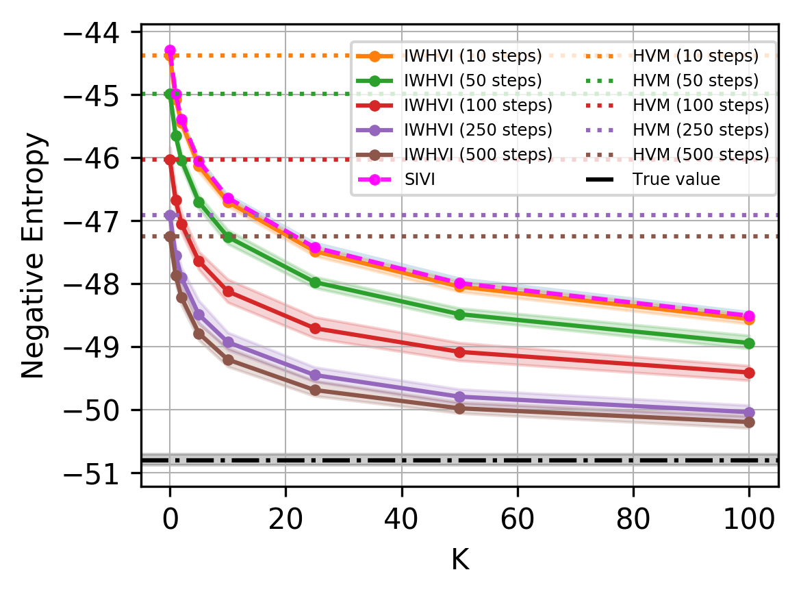Comparison of IWHVI bounds for different number of optimization steps over $\eta$.

Moreover, multisample bounds have been extensively studied and some results translate to our bound as well.

Estimating the marginal log-likelihood $\log p_\theta(x)$

Increasing $K$ will lead to the bound $\hat{\mathcal{L}}_K^\text{IWHVI}$ approaching the ELBO $\mathcal{L}$, but the gap between the ELBO and the marginal log-likelihood $\log p_\theta(x)$ is not negligible. Even by employing more powerful variational distribution we might not be able to overcome the gap introduced by amortization. The standard approach to evaluate Variational Autoencoders it to use the Multisample Variational Lower Bound (IWAE bound) with large $M$. Can we tighten our bound in such a way?

It turns out, the answer is yes and the tighter bound is simply

$$ \hat{\mathcal{L}}_K^\text{$M$-IWHVI} := \E_{\substack{q_\phi(z_{1:M}, \psi_{1:M, 0}|x) \\ \tau_\eta(\psi_{1:M, 1:K}|z_{1:M}, x)}} \log \frac{1}{M} \sum_{m=1}^M \frac{p_\theta(x, z_m)}{ \frac{1}{K+1} \sum_{k=0}^K \frac{q_\phi(z_m, \psi_{m,k}|x)}{\tau_\eta(\psi_{m,k}|x,z_m)} } \le \log p_\theta(x) $$

Essentially we just sampled the original $\hat{\mathcal{L}}_K^\text{IWHVI}$ bound $M$ times (independently) and averaged them all inside the $\log$.

But Tighter Variational Bounds are Not Necessarily Better

It was observed that training IWAE with large $K$ leads to inference networks gradients deterioration. Namely, the signal-to-noise ratio of $\nabla_\phi \mathcal{L}_K$ estimates decrease with $K$, while the signal-to-noise ratio of $\nabla_\theta \mathcal{L}_K$ estimates increase with $K$. Luckily, the Doubly Reparameterized Gradients paper resolved this problem. The same derivations apply to our case except for having an additional term corresponding to a sample from $q_\phi(\psi|z, x)$, which prevents SNR from increasing, leaving it approximately constant.

Debiasing and Jackknife

Nowozin has shown that Multisample Variational Lower Bound $\mathcal{L}_K$ (the IWAE bound) can be seen as a biased evidence estimate with the bias of order $1/K$, which can be reduced with Jackknife. This procedure results in an improved estimator with the bias of order $1/K^2$. By repeating the procedure over and over again $d$ times we obtain an estimator with the bias of order $1/K^{d+1}$. The price for that is increased variance, computational complexity and loss of bound guarantees.

It can be shown that the Multisample Variational Upper Bound $\mathcal{U}_K$ also has the bias of order $1/(K+1)$ and thus allows the jackknife. We tested the debiased estimator on a toy task but did not use it in more serious experiments due to loss of guarantees.

Is SIVI obsolete?

It depends. In the case of Neural Samplers IWHVI does give a much tighter bound with little extra overhead. However, in some cases the general formulation of IWHVI might be challenging to work with, for example, in the case of VampPrior-like distributions: $$ q_\phi(z) := \frac{1}{N} \sum_{n=1}^N q_\phi(z|x_n) = \sum_{n=1}^N q_\phi(z|n) q(\psi = n) $$ Here $\psi$ is essentially a number from 1 to N and the prior $q(\psi)$ is a uniform distribution. The IWHVI bound would involve $\tau(\psi|x,z)$ as a categorical distribution over $N$ outcomes. Learning $\tau$ not only would require advandced gradient estimates² to deal with discrete random variables, but also an efficient softmax estimators to scale favorably to large datasets. In this setting SIVI presents a much simpler alternative as it frees us from all these hurdles. SIVI only requires sampling from $U\{1, \dots, N\}$, which is easy.

In many cases though, IWHVI only adds one extra pass of each $z$ through a network that generates $\tau_\eta(\psi|z,x)$ distribution, which is dominated by $K+1$ passes of $\psi_{0:K}$ through a network that generates $q_\phi(z|x, \psi_k)$ distributions, so it's added cost is negligible.

Conclusion

In this work we identified a generalized bound that bridges prior work on HVM and SIVI. Such generalized bounds are shown to be much tighter. A particularly nice property is that such multisample bound breaks the vicious cycle we stumbled upon in the last post: increasing the number of samples allows us to tighten the bound without complicating the auxiliary variational distribution $\tau_\eta(\psi|x,z)$ and thus reduce the amount of regularuzation simple it imposes on the true inverse model $q_\phi(\psi|x,z)$, which lets us learn expressive Neural Samplers. Although multiple samples are still more computationally expensive than just one sample (HVM), $z$ typically has much lower dimension than $x$, so this bound is cheaper to evaluate than the IWAE's one.

For more details check out the preprint.