This is the second post of the stochastic computation graphs series. Last time we discussed models with continuous stochastic nodes, for which there are powerful reparametrization technics.

Unfortunately, these methods don't work for discrete random variables. Moreover, it looks like there's no way to backpropagate through discrete stochastic nodes, as there's no infinitesimal change of random values when you infinitesimally perturb their parameters.

In this post I'll talk about continuous relaxations of discrete random variables.

Asymptotic reparametrization

One way to train models with discrete random variables is to consider an equivalent model with continuous random variables. Let me show you an example. Suppose you have a feed-forward neural network for classification that receives $x$ and outputs distribution over targets $p(y \mid x)$, where typical layer looks like $h_k = \sigma(W_k h_{k-1} + b_k)$. You'd like to apply dropout to each weight of this layer and tune its probabilities. To do so we introduce binary latent variables $z^{(k)}_{ij}$ denoting if weight is on or off. There's one such variable for each weight, so we can stack them into a matrix $Z_k$ of the same shape as weight matrix $W_k$. Then element-wise multiplication $W_k \circ Z_k$ would zero out dropped weights, so the formula becomes $h_k = \sigma((W_k \circ Z_k) h_{k-1} + b_k)$. We assume each dropout mask independently follows Bernoulli distribution: $z_{ij}^{(k)} \sim \text{Bernoulli}(p_{ij}^{(k)})$ ($Z^{(k)} \sim \text{Bernoulli}(P^{(k)})$ for short)

In order to learn these masks (or, rather parameters of the distribution $q(Z \mid \Lambda)$ over masks parametrized by $\Lambda$) we employ variational inference approach:

$$ \begin{align*} \log p(y|x) \ge \mathcal{L}(\Lambda) &= \mathbb{E}_{q(Z \mid \Lambda)} \log \frac{p(y, Z \mid x)}{q(Z \mid \Lambda)} \\ &= \underbrace{\mathbb{E}_{q(Z \mid \Lambda)} \log p(y \mid Z, x)}_{\text{expected likelihood}} - \underbrace{D_{KL}(q(Z \mid \Lambda) \mid\mid p(Z))}_{\text{KL-divergence}} \to \max_\Lambda \end{align*} $$

We can't backpropagate gradients through discrete sampling procedure, so we need to overcome this problem somehow. Notice, however, that each unit in a layer $h_{k+1}$ is an affine transformation of $k$th layer's nodes followed by a nonlinear activation function. If $k$th layer has sufficiently many neurons, then one might expect the Central Limit Theorem to hold at least approximately for the preactivations. Namely, consider a single neuron $s$ that takes an affine combination of previous layer's neurons $h_{k-1}$ and applies a nonlinearity: $s = \sigma(w^T h + b)$. In our case, however, we have a vector of masks $z \sim \text{Bernoulli}(P)$, so the formula becomes $s = \sigma((w \odot \tfrac{z}{P})^T h + b)$ ($\odot$ stands for element-wise multiplication), and if $K=\text{dim}(z)$ is large enough, then we might expect the preactivations $\sum_{k=1}^K \tfrac{z_k}{p_k} w_k h_k + b$ (we divide each weight by its keeping probability $p_k$ to make keep the expectation unaffected by noise) to be approximately distributed as $\mathcal{N}\left(w^T h + b, \sum_{k=1}^K \tfrac{1 - p_k}{p_k} w_k^2 h_k^2 \right)$.

Now suppose that instead of Bernoulli multiplicative noise $z$ we actually used multiplicative Gaussian noise $\zeta \sim \mathcal{N}(1, (1-P) / P)$ (element-wise division). It's easy to check then that the preactivations $(w \odot \zeta)^T h + b$ would have the same Gaussian distribution with exactly the same parameters. Therefore, we can replace expected likelihood term in objective $\mathcal{L}(\Lambda)$ with a continuous distribution $q(\zeta|\Lambda) = \prod_{i,j,k} \mathcal{N}\left(\zeta^{(k)}_{ij} \mid 1, (1-\lambda^{(k)}_{ij})/\lambda^{(k)}_{ij}\right)$. However, we can't simply do the same in the KL divergence term. Instead, we need to use simple priors (like factorized Bernoulli) so that closed form can be computed – then we can take deterministic gradients w.r.t. $\Lambda$.

This example shows us that for some simple models collective behavior of discrete random variables can be accurately approximated by continuous equivalents. I'd call this approach the asymptotic reparametrization ¹.

Naive Relaxation

The previous trick is nice and appealing, but has very limited scope of applicability. If you have just a few discrete random variables or have other issues preventing you from relying on the CLT, you're out of luck.

However, consider a binary discrete random variable: $z \sim \text{Bernoulli}(p)$. How would you sample it? Easy! Just sample a uniform r.v. $u \sim U[0,1]$ and see if it's less than $p$: $z = [u > q]$ where $q = 1 - p$ and brackets denote an indicator function that is equal to one when the argument is True, and zero otherwise. Equivalently we can rewrite it as $z = H(u - q)$ where $H(x)$ is a step function: it's zero for negative $x$ and 1 for positive ones ². Now, this is a nice-looking reparametrization, but $H$ is not differentiable ³, so you can't backpropagate through it. What if we replace $H$ with some differentiable analogue that has a similar shape? One candidate is a sigmoid with temperature: $\sigma_\tau(x) = \sigma\left(\tfrac{x}{\tau}\right)$: by varying temperature you can control steepness of the function. In the limit of $\tau \to 0$ we actually recover the step function $\lim_{\tau \to 0} \sigma_\tau(x) = H(x)$.

So the relaxation we'll consider is $\zeta = \sigma_\tau(u - q)$. How can we see if it's a good one? What do we even want from the relaxation? Well, in the end we'll be using the discrete version of the model, the one with zeros and ones, so we'd definitely like our relaxation to sample zeros and ones often. Actually, we'd even want them to be the modes of the underlying distribution. Let's see if that's the case for the proposed relaxation.

CDF of the relaxed r.v. $\zeta$ $$ \mathbb{P}(\zeta < x) = \mathbb{P}(u < q + \tau \sigma^{-1}(x)) = \min(1, \max(0, q + \tau \sigma^{-1}(x))) $$ And the corresponding PDF $$ \frac{\partial}{\partial x}\mathbb{P}(\zeta < x) = \begin{cases} \frac{\tau}{x (1-x)}, & \sigma\left(\frac{-q}{\tau}\right) < x < \sigma\left(\frac{1-q}{\tau}\right) \\ 0, & \text{otherwise} \end{cases} $$

Even the formula suggests that the support of the distribution of $\zeta$ is never the whole $(0, 1)$, but only approaches it as temperature $\tau$ goes to zero. For all non-zero temperatures though the support will exclude some neighborhood of the endpoints which might bias the model towards the intermediate values. This is why you want to have a random variable with infinite support ⁵. If the distribution is skewed, then the resulting relaxation will also be skewed, but it's not a problem since the probabilities are adjusted according to the CDF.

Let's plot some densities for different $\tau$ (let $q$ be 0.1).

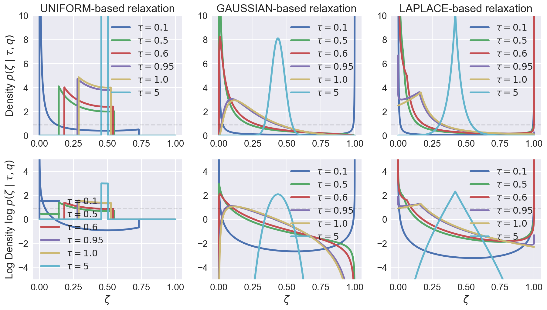
But having infinite support is not enough. It's hard to see from plots, but if the distribution has very light tails (like Gaussian), then it's effective support is still finite. Authors of the Concrete Distribution notice this in their paper, saying that sigmoid squashing rate is not enough to compensate (even if you twist the temperature!) for density decrease as you approach either of infinities.

Let's also think about the impact of the temperature on the relaxation. Intuitively one would expect that as we decrease the temperature, the relaxation becomes more accurate and the problem becomes "more discrete", hence it should be harder to optimize. Indeed, $\tfrac{d}{dx}\sigma_\tau(x) = \tfrac{1}{\tau} \sigma_\tau(x) \sigma_\tau(-x)$ – as you decrease the temperature, both sigmoids become more steep, and the derivative approaches an infinitely tall spike at 0 and zero everywhere else ⁴.

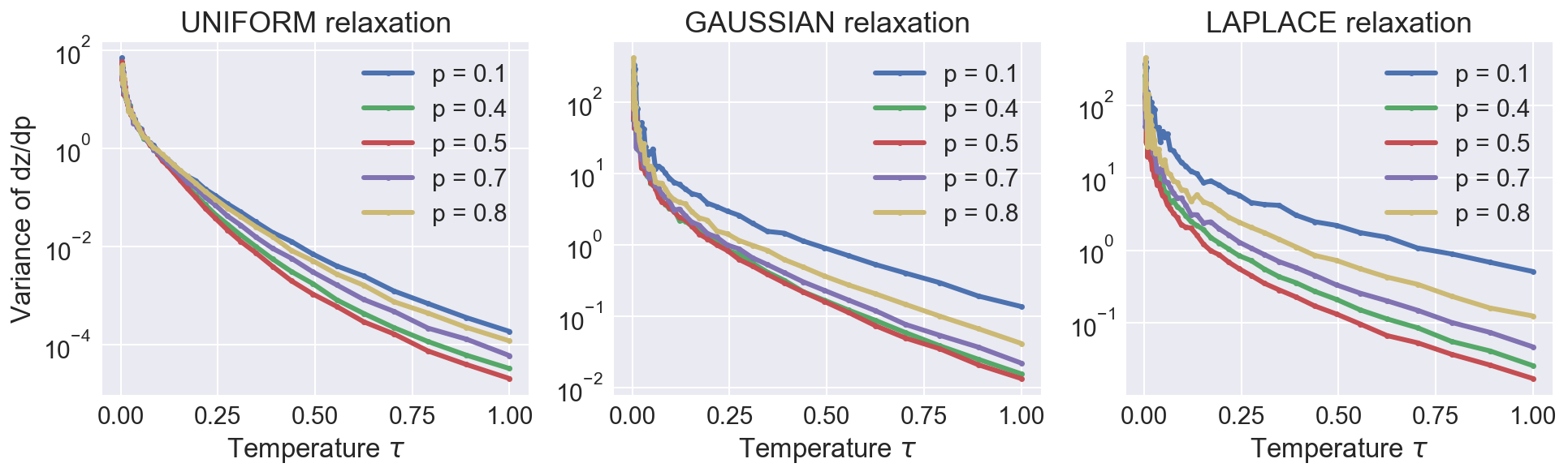
As expected, higher approximation accuracy (obtained by lowering the temperature) comes at a cost of increased variance.

Gumbel-Softmax Relaxation (aka Concrete Distribution)

We could consider some other distributions (with larger support, like the gaussian one) instead of uniform in our relaxation, but let's try a different approach. Let's see how we can sample arbitrary $K$-valued discrete random variables. It's well-known fact (the so called Gumbel Max Trick) that if $\gamma_k$ are i.i.d. $\text{Gumbel}(0, 1)$ random variables, then $\text{argmax}_k \{\gamma_k + \log p_k\} \sim \text{Categorical}(p_1, \dots, p_K)$, that is, probability that $k$th perturbed r.v. attains maximal value is exactly $p_k$ ⁶. This gives you a sampling procedure: just sample $K$ independent Gumbels, add corresponding log probabilities, and then take the argmax. However, though mathematically elegant, this formula won't help us much since argmax is not differentiable. Let's relax it then! We have already seen that the step function $H(x)$ can be seen as a limit of a sigmoid with temperature: $H(X) = \lim_{\tau \to 0} \sigma_\tau(x)$, so we might expect (and indeed it is) that if you assume that $\text{argmax}(x)$ returns you a one-hot vector indicating the maximum index, it can be viewed as a zero-temperature version of a softmax with temperature: $\text{argmax}(x)_j = \lim_{\tau \to 0} \text{softmax}_\tau(x)_j$ where

$$ \text{softmax}_\tau(x)_j = \frac{\exp(x_j / \tau)}{\sum_{k=1}^K \exp(x_k / \tau)} $$

This formula gives us continuous relaxation of discrete random variables. Let's see what it corresponds to in binary case:

$$ \begin{align*} \zeta &= \frac{\exp((\gamma_1 + \log p) / \tau)}{\exp((\gamma_1 + \log p) / \tau) + \exp((\gamma_0 + \log (1-p)) / \tau)} \\ &= \frac{1}{1 + \exp((\gamma_0 + \log (1-p) - \gamma_1 - \log p) / \tau)}\\ &= \sigma_\tau\left(\gamma_1 - \gamma_0 + \log \tfrac{p}{1-p}\right) \end{align*} $$

Then $\gamma_1 - \gamma_0$ has Logistic(0, 1) distribution ⁷. This estimator is a bit more efficient since you can generate Logistic random variables faster than generating two independent Gumbel r.v.s. ⁸

Even though this choice of Logistic distribution in binary case seems arbitrary, let's not forget, that it's a special case of a more general relaxation of any categorical r.v. If we chose some other⁵ distribution in a binary case, we'd have to construct some cumbersome stick-breaking procedure to generalize it to the multivariate case.

Marginalization via Continuous Noise

An interesting approach was proposed in the Discrete Variational Autoencoders paper. The core idea is that you can smooth binary r.v. $z$ with p.m.f. $p(z)$ by adding extra noise $\tau_1$ and $\tau_2$ and treating $z$ as a swticher between these. Indeed, consider such smoothed r.v. $\zeta = z \cdot \tau_1 + (1 - z) \tau_0$. Now if we choose $\tau_0$ and $\tau_1$ such that the CDF of marginal $\zeta$ can be computed and inverted, we would be able to devise a reparametrization for this scheme.

Consider a particular example of $\tau_0 = 0$ – a constant zero, and $\tau_1$ having some continuous distribution. The marginal CDF of $\zeta$ would then be

$$ \mathbb{P}(\zeta < x) = \mathbb{P}(z = 0) [\zeta > 0] + \mathbb{P}(z=1) \mathbb{P}(\tau_1 < x) $$

Now we can invert this CDF:

$$ \mathbb{Q}_\zeta(\rho) = \begin{cases} \mathbb{Q}_\tau \left( \frac{\rho}{p(z=1)} \right), & \rho \le p(z=1) \mathbb{P}(\tau < 0) \\ \mathbb{Q}_\tau \left( \frac{\rho - p(z = 0)}{1 - p(z = 0)} \right), & \rho \ge p(z = 0) + p(z=1) \mathbb{P}(\tau < 0) \\ 0, & \text{otherwise} \end{cases} $$

Where $\mathbb{Q}_\tau(\rho)$ is an inverse of CDF of $\tau$, that is $\mathbb{P}(\tau < \mathbb{Q}_\tau(\rho)) = \rho$. This formula clearly suggests that if you can compute and invert CDF of the smoothing noise $\tau$, you can do the same with the smoothed variable $\zeta$, essentially giving us reparametrization for the smoothed r.v. $\zeta$, so we can backpropagate as usual. ¹⁰

However, an attentive reader could spot a problem here. In the multivariate case we typically have some dependency structure, hence probabilities $p(z_k = 0)$ and $p(z_k = 1)$ depend on previous samples $z_{<k}$, which we can't backpropagate through, and need to relax in the same way.

Consider, for example, a general stochastic computation graph with 4-dimensional binary random variable $z$:

When applying this trick, we introduce relaxed continuous random variables $\zeta$ as simple transformations of corresponding binary random variables $z$ (red lines), and make $z$ depend on each other only through relaxed variables (purple lines).

This trick is somewhat similar to the asymptotic reparametrization – you end up with a model that only has continuous random variables, but is equivalent to the original one that has discreteness. However, it requires you to significantly alter the model by re-expressing dependence in $z$ using continuous relaxations $\zeta$. It worked fine for the Discrete VAE application, where you want to learn this dependence structure in $z$, but if you have a specific one in mind, you might be in trouble.

Also, we don't want to introduce this noise at the test stage. So we'd like to fix the discrepancy between train and test somehow. One way to do so is to choose $\tau$ that depends on some parameter and adjust it so that $\tau$'s distribution becomes closer to $\delta(\tau-1)$. In the paper authors use "truncated exponential" distribution $p(\tau) \propto \exp(\beta \tau) [0 \le \tau \le 1]$ where $\beta$ is a (bounded) learnable parameter. The upper bound grows linearly as training progresses – essentially shrinking the noise towards 1 (in the limit of infinite $\beta$ we have $p(\tau) = \delta(\tau-1)$).

Gradient Relaxations

There's been also some research around the following idea: we don't have any problems with discrete random variable during the forward pass, it's differentiation during the backward one that brings difficulties. Can we approximate the gradient only? Essentially the idea is to compute the forward pass as usual, but replace the gradient through random samples with some approximation. To a mathematician (like I pretend to be) this sounds very suspicious – the gradient will no longer correspond to the objective, it's not even clear which objective it'd correspond to. However, these methods have some attractive properties, and are well-known in the area, so I feel I have to cover them as well.

One of such methods is the Straight Through estimator, which backpropagates the gradient $\nabla_\theta$ through binary random variable $z \sim \text{Bernoulli}(p(\theta))$ as if there was no stochasticity (and nonlinearity!) in the first place. So in the forward pass you take your outputs (logits) of a layer preceding to the discrete stochastic node, squash it by a sigmoid function, then sample a Bernoulli random variable with such probability, and move on to the next layer, possibly sampling some more stochastic nodes along the way. In the backward phase, though, when it comes to differentiate through the discrete sampling procedure, you just go straight to the gradients of logits, like if there was no sigmoid and sampling in the first place: $$\nabla_\theta \text{Bernoulli}(\sigma(g(\theta))) := \nabla_\theta g(\theta)$$

This estimator is clearly computing anything but an estimate of the gradient of your model, but authors claim that at least it gives you right direction for the gradient. You can also keep the sigmoid function – that's what Raiko et. al do: $$\nabla_\theta \text{Bernoulli}(\sigma(g(\theta))) := \nabla_\theta \sigma(g(\theta))$$

Finally, authors of one of the Gumbel-Softmax relaxation papers proposed Straight Through Gumbel where you, again, compute forward pass as usual, but in the backward pass assume there's Gumbel-Softmax relaxation and backpropagate through it. Hypothetically as you decrease the temperature, this relaxation becomes more exact. I guess one can try to convince themselves that for small enough $\tau$ this is a reasonable approximation. $$\nabla_\theta \text{Bernoulli}(\sigma(g(\theta))) := \nabla_\theta \text{RelaxedBernoulli}(\sigma(g(\theta)))$$

I personally consider these methods mathematically unsound, and advise you to refrain form using them (unless you know what you're doing – then tell me what was your rationale for this particular choice).

Experiments

To please your eyes with some experimental plots, I used all these relaxations to train a Discrete Variational Autoencoder on MNIST. I used a single stochastic layer (shallow encoder) with 3 layers in between, and evaluated the result using 10,000-sample lower bound, which I assume approximates marginal log-likelihood relatively well.

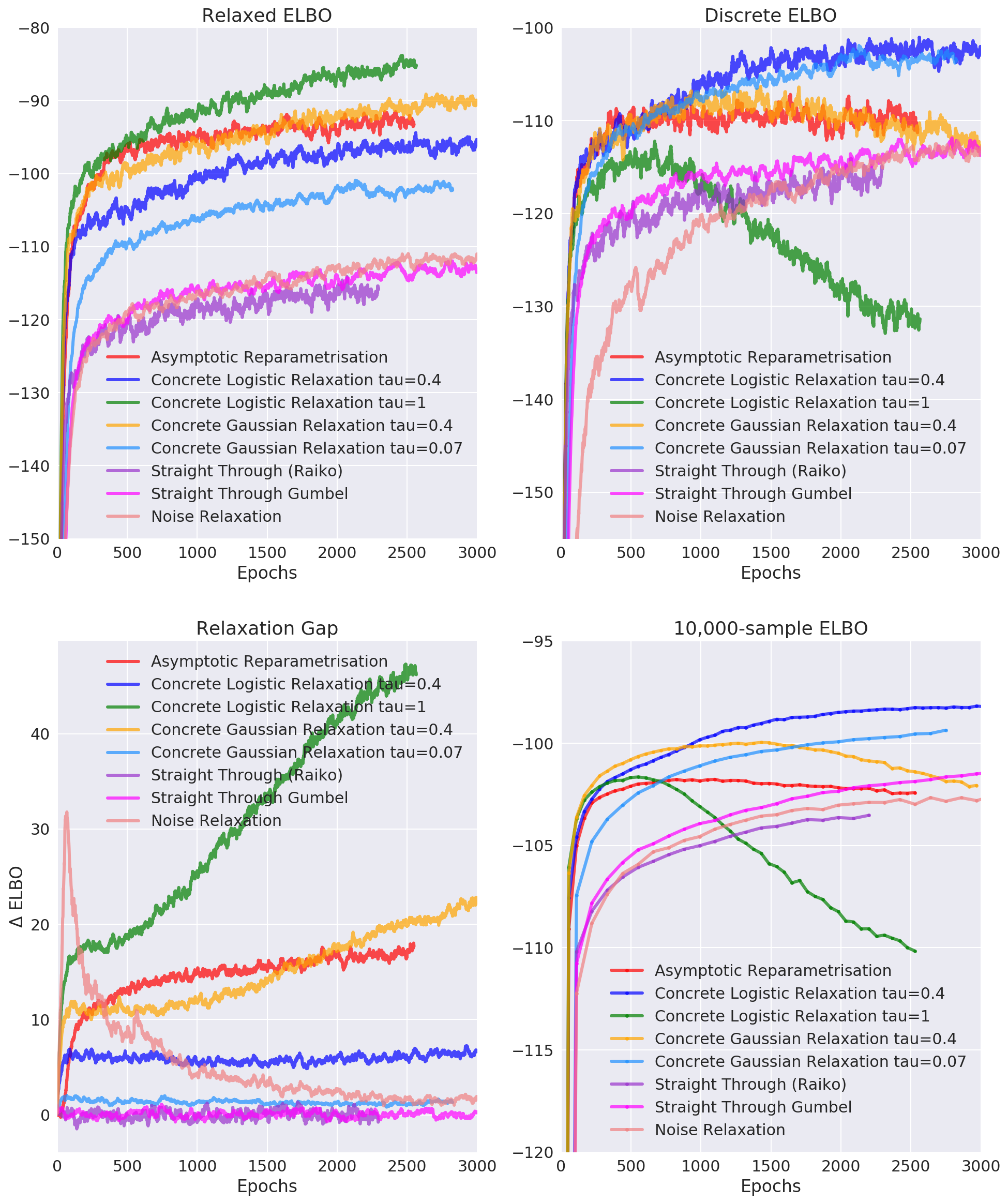
First, the Relaxed ELBO pane tells us all methods have no problems optimizing their target objective. However, one should refrain from comparing them according to this number, since these are different relaxations, they are not even lower bounds for a marginal log-likelihood for some relaxed model ¹¹.

Instead, let's look at the second and third panes. The second shows the Evidence Lower Bound for the original discrete model, and the third shows the gap between the discrete ELBO and the relaxed one. First, the marginal likelihood estimation agrees with the discrete ELBO – that's a good thing and means nothing bad is happening to the KL-divergence between the true posterior and the approximate one.

You can see that the green line – the logistic distribution-based relaxation with unit temperature – actually diverges. This is a direct consequence of the chosen temperature: for $\tau = 1$ the density of relaxed random variables is unimodal and has its mode somewhere in the interior of the [0, 1] interval. This leads the network to adjust to the values around this mode, which poorly represent test time samples.

As you can see the normal distribution with temperature 0.4 works very well at first, but then starts diverging. This might be because of the problems of Gaussian distribution we discussed earlier: namely, it has zero mass at exact 0 and 1: the network might adapt to having some small non-zero elements, and be very surprised to see them zeroed out completely at the testing time.

The asymptotic reparametrization seems to be suffering from the inaccuracy of the CLT approximation. Latent code of 200 units is big, but not infinitely big for the approximation to be exact. Unfortunately, there's no hyperparameter to adjust the approximation quality. Moreover, the relaxation gap keeps increasing.

The Noise-Relaxed model performs poorly compared to other methods. This might be a result of a poor hyperparameter management: recall that we introduce continuous noise that's missing at the test time. To make the net adjust to the test time regime we need to make the noise approach $\delta(\tau - 1)$. However, if you approach it too fast, you'll see the relaxation gap decreasing, but the learning wouldn't progress much as the variance of your gradients would be too high.

Straight through estimators perform surprisingly good: not as good as the Gumbel-Softmax relaxation, but better than what you'd expect from a mathematically unsound method.

Conclusion

In this post we talked about continuous relaxations of discrete models. These relaxations allow you to invoke the reparametrization trick to backpropagate the gradients, but this comes at a cost of bias. The gradients are no more unbiased as you essentially optimize different objective. In the next blogpost we will return back to where we started – to the score-function estimator, and try to reduce its variance keeping zero bias.

By the way, if you're interested, the code for DVAE implementations is available on my GitHub. However, I should warn you: it's still work-in-progress, and lacks any documentation. I'll add it one I'm finished with the series.